
Ok, so I’ve done a lot of preparatory stuff in Part 1 (building a swing and understanding a pendulum) where I pushed Marty to get him swinging and Part 2 (making a swing simulator that models the increase in system energy from pumping the swing). Now I get to the good stuff and answer the question: “how does Marty (or at least Sim-Marty) actually LEARN to swing”?
To do this I’m going to explore and implement a learning technique called Q-Learning. Although the idea of a machine learning something might seem like science fiction the idea and reality of Q-Learning is pretty simple. First I’ll delve a little into what Q-Learning is and then I’ll implement some Q-Learning code to get Sim-Marty to learn to swing.
Q-Tables
A core element of Q-Learning is the Q-Table and it’s a simple idea. A Q-Table is essentially a cheat-sheet that tells you (or a robot) what to do for the best outcome in any of the situations a simulation (or real-world system) can get into. For instance, a Q-Table for walking to the shops might look something like this:
| Current Location | Walk Straight | Turn Left | Turn Right |
|---|---|---|---|
| Home | 1 | 0 | 0 |
| Outside Front Door | 0 | 1 | 0 |
| My Street | 1 | 0 | 0 |
| Corner of My Street and Main Road | 0 | 0 | 1 |
| Main Road | 1 | 0 | 0 |
| Outside Shop | 0 | 0 | 1 |
To follow the instructions in the table you determine where you currently are (I will call this your current “state”) and then look-up the row in the table that corresponds to that state. Next look along that row and find the column with the highest number in it. Then choose the action corresponding to that column.
Pretty simple right!
I have to confess my example Q-Table above isn’t perfect as you should be able to use it starting from any location but my instructions presume that you are facing in a particular direction (but you get the idea I hope).
There are some limitations to the kind of problems that can be solved with Q-Tables but, generally speaking, as long as you can define a specific action to take in each situation and what you did previously has no bearing on which is the best action to take right now, then a Q-Table can be used.
Building a Q-Table Randomly
The great thing about Q-Tables is that once you have a complete one for your “problem” all you need to do is follow the method above and you will be able to take the best action in every situation. However, a difficulty arises in writing down the Q-Table if you don’t know what the best action is before you start. So in that case how can you build a Q-Table?
One technique you could employ is a “random-walk”. Let’s say you have a lot of time on your hands and you want to find the local shop in an area you don’t know (but you do know that only two turns are necessary – because your friend told you so).
One thing you could do is to walk in a random direction from the starting point and then carry on until you reach a turning point. You could then choose a random direction from there and carry on until you either reach the shop or another turning point.
If you didn’t reach the shop you now need to turn back (your friend told you only two turns were needed) and walk back to the last turn you made and then choose a random direction. Continue again until you either find the shop or hit a turning point. Then repeat this paragraph until you get too tired (or find the shop!).
Now (assuming you didn’t find the shop) you go back to where you started and choose a random direction from there. Eventually you will (probably) find the shop and you could then write the perfect Q-Table based on your experiences.
This kind of method actually has a name – it is called a Monte Carlo method because it uses random luck – and is (perhaps surprisingly) used quite often for building Q-Tables – believe it or not! It may seem extremely inefficient – I mean why not just remember where you had been each time and choose a different direction to walk in – surely that would be better.
Well, of course, that would be better but it would both require a lot of remembering where you had been and it would only work if the direction was a “discrete” quantity – like “left”, “right”, “straight-on”, etc. If the direction is a compass bearing to five decimal places then it won’t really work to try every possible bearing you’ve tried – and imagine how big the Q-Table would need to be to accommodate all of those directions.
The Big-Idea of Q-Learning
Q-Learning actually uses a method similar to the above. The only real difference is that in Q-Learning the Q-Table is updated continually as you go along whereas in the example above we learned everything first and then wrote the perfect Q-Table at the end.
The big-idea of Q-Learning is that we can evaluate how good an action is after we have taken it by considering whether the place it gets us to is in the direction of our goal. The value of an action is determined by the idea of a “reward” that we get from having taken the action. In the case of trying to find the local shop the only reward we can get is when we actually find the shop. Until we actually get there it isn’t possible to say whether we are on the right path.
This might sound like it assumes we have to know the directions already and, in fact, there is an element of truth in this because you need to have found some reward (by randomly trying things) before you can start to determine which path leads to the best reward. Q-Learning is really a way to reinforce the knowledge of a path already found rather than a way to find the path in the first place. Ultimately there is no clever method in Q-Learning for finding a path – you simply have to stumble upon it by trying lots of things randomly! Of course other clever methods could be used to predict where the shop was if you had more information but Q-Learning simply assumes that some random actions will be taken and that eventually the best set of actions in each state will emerge as the better paths are reinforced and the less good ones are diminished.
There’s a much more complete explanation of Q-Learning in this post.
Implementing Q-Learning for the Sim-Marty
In Part 2 I implemented an OpenAI Gym to simulate Marty on a Swing and defined two actions that could be taken at each step of the simulation:
- Kick – Marty bends his knees
- Straight – Marty straightens his knees
The gym gives back one piece of information about the state of the Marty Swing at each step and we need to use that information (and nothing else) to make a decision about whether to Kick or Straight-en Marty’s legs. That piece of information is the simulated reading from Marty’s accelerometer (X-Axis) – I will call this value xAcc – and it is an indication of how much Marty is accelerating in a direction which corresponds to Marty’s swing. From Part 1 we also know that this is also related to where in the swing Marty currently is:
- high (positive) xAcc value means Marty is close to one of the limits of his swing (high point 1)
- close to zero xAcc value means Marty is near the middle of his swing
- lowest (negative) xAcc value means Marty is close to the other of the limits of his swing (high point 2)
Since xAcc is closely related to the angle that Marty is currently at we can simply use it as a “proxy” for the angle of Marty’s swing. With zero indicating straight-down and the positive and negative maximum values that xAcc reaches indicating the limits of the angle of swing in each direction.
Turning Acceleration into a Discrete Value
I mentioned above that Q-Tables are only any good when the “state” is a discrete quantity (taking one of a finite set of values) and with relatively few possible values (otherwise the Q-Table would be huge). But acceleration is continuous (it can have any value within a range to a significant number of decimal places) so I need to reduce the set of possible values of xAcc without losing its meaning.
Fortunately I think we can assume that it won’t really matter that Marty starts an action exactly at a specific point on his swing, just as it doesn’t really matter exactly when you lean back on a playground swing. As long as Marty pumps at approximately the right position all will be fine.
So I will consider the xAcc value to be like the angle of swing and then I can imagine his swing split into a number of segments (of a circle centered on his swing axis) and decide what action to take based on which segment Marty is current in. After trying a few different numbers of segments I decided to go with 9 (or 18 in total if both directions of swing are counted).
The segment idea should become clearer when looking at the animation below (I’m only showing the 7 segments that are below the horizontal line through the swing axis for clarity). The other two segments would only come into play if Marty learned to swing so high that he went above the axis pole.
Starting up Q-Learning
The program file martySwingGymQLearn.py implements Q-Learning for Marty. I started the program based on this article, and, while there isn’t much of the original code left, the general idea remains the same. The following animations (generated by the program martySwingGymLearnGIF.py which has the additional code to generate the GIF file) shows the start of the Q-Learning process.

In the animation the top line of colored dots indicates the behavior of Marty when swinging right-to-left and the lower line is for left-to-right. The color codes are as follows:
- yellow: Marty hasn’t reached this segment yet (so we haven’t learned what to do)
- red: the Q-Table for this state indicates that Marty should have Kicked legs at this point in his swing
- green: the Q-Table indicates Marty should have Straight legs at this point
At this point in Marty’s training he doesn’t know whether to kick or straighten at any point as he hasn’t received much information (rewards) to tell him when he is doing well. But as you watch the animation play-out you will see some of the dots change color. At this stage of learning this happens quite a lot and the rate can be controlled by a variable in the program called learningRate. Initially this is set to 1.0 (full-learn-mode!) and then, as Marty starts to learn, it is reduced (to a minimum of 0.1) so that he tends to reinforce previously good learning rather than just trashing it constantly.
You can also see from the swing angle chart that Marty isn’t gaining (or losing) much height in his swing – he hasn’t yet learned how to swing.
Learning Progression
As described above Q-Learning involves sometimes taking random actions instead of the ones Marty currently think are best. In my program the amount of randomness in decision making is determined by a variable called explorationRate which starts with a value of 1.0 (full-explore-mode!) and reduces to 0.01 as learning progresses. What this means in practice is that at the start of learning almost all actions are random and Marty explores lots of possible actions, but later on Marty stops being so inquisitive and starts to just try the odd different action from time to time.

Watching this animation (which was created after Marty had done about 10 practice runs) you will see that the colors of the dots change less frequently than before. This is because the learning rate has slowed and Marty is starting to reinforce the pattern of swinging which is giving him the best rewards.
You may also notice from the Swing Angle chart that there is a slight increase in swing angle on each swing – don’t worry if you can’t see it as it is very slight at present. This is an indication that Marty is homing-in on a good swinging strategy and, left to practice a few more times he will start to get quite good.
When to Stop Learning
Here’s the result of Marty practicing swinging around 100 times.

You should be able to see from the Swing Angle chart that Marty is now getting quite good at swinging as each cycle is a little bigger than the last. The colors of the dots also now aren’t changing at all, he’s locked-into a swing strategy that works well enough because the learning rate and exploration rate have become very low.
If you were to ask whether he is swinging as well as is possible then the answer would almost certainly be “no” – he could do better. But essentially he’s stopped trying different ways to swing because he’s decided he is good enough already.
Randomness, Learning Rate and Good Enough Swinging
So I now have a program which allows Marty to try-out different swinging patterns (which I called strategies) and learn which ones work well enough. If I were to run the same program multiple times (and believe me I have!) then I will get a different result every time. Sometimes Marty learns quickly and finds a very good swinging pattern but at other times it takes him a lot longer to find something good.
The three charts above are from three runs of the training process with exactly the same parameters.
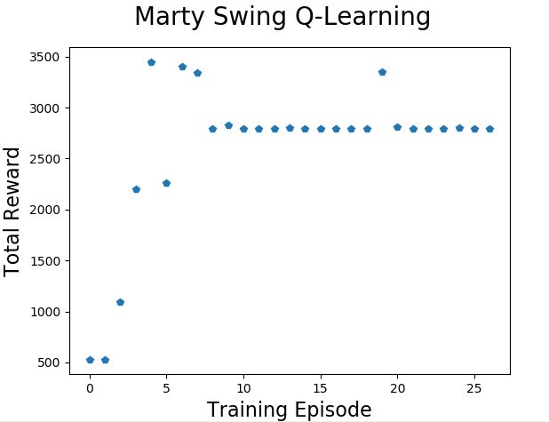
In this run Marty learned to swing very quickly and held onto the pattern long enough to convince us that he had learned well (ten consecutive swings above a total reward of 2500).
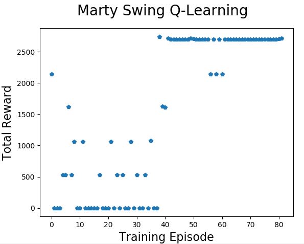 On this run Marty found some early ways to get total rewards in the range 500 to 2200 but it took quite a few more training practices to get consistently up above the 2500 level. And even once he had done that he still experimented with some less-good pattern changes that lost him the chance to complete the task early.
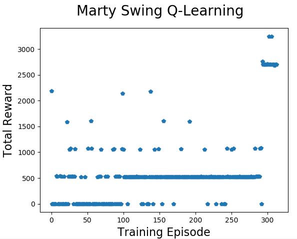
This was one of the worst runs I recorded and shows that it is possible for Marty to get stuck on a pattern that isn’t very good. The fact that the exploration rate and learning rate both reduce quickly also means that when Marty has practiced 250 times he isn’t exploring that much and isn’t learning very fast – which makes it hard to get past the poor pattern and find a better one.
Endlessly Tweaking the Hyperparameters
Practically speaking it is possible to improve the Q-Learning method by changing the parameters around learning rate, exploration rate, discount and reward-shape (and probably other things). The first two items have been explained above it probably makes sense by now that changing the starting, ending and rate of change of these values would affect the way Marty explores and learns.
The latter two parameters are to do with how rewards are applied during learning and what value the rewards take. The discount rate is used in the Bellman equation (described in this video) and can be tuned to set how long after an action is taken the reward might be expected to appear. In the first version of the Marty swing gym I decided to give a large positive reward based on swinging higher than the previous cycle and a small negative reward each time Marty kicked. This seemed to work out OK but I then tried removing the negative reward and, for some reason I’m not quite clear on, this seemed to work better.
The fact is that tweaking (changing) these parameters makes a big difference to how well (on average) Q-Learning works. Since the learning process is somewhat random there is always also some difference in how the learning process performs on each run. I’ve spent a lot of time trying to find sensible values for these parameters and I think it might be sensible to look at a genetic algorithm to try to optimize them – but instead I’m going to take a different approach altogether and try to make things more “deterministic” (or less random).
Exploring Every Possible Swing Pattern
In Q-Learning results vary from run to run so it is quite difficult to say how many runs it will take to come up with a good solution to the swinging pattern. What I have decided to do is, instead of letting the Q-Learning algorithm randomly change the pattern until it find something good, I’m going to try out every possible pattern and then choose the best one.
But won’t that be billions of different patterns to try though?
Well, since I have already reduced the number of segments to 5 (actually there are 9 but you can see from the animations that in normal conditions only 5 of them are really used) and there are two directions then there are just 10 points in Marty’s swing where there is a choice actions to be taken. At each of these 10 places there are two potential actions so the total number of permutations (alternative patterns) of actions is only 1024.
We’re actually doing a few hundred runs in any case and not getting to the very best answer each time so if we exhaustively try every one of the 1024 different patterns then we’ll know the very best pattern of swinging.
To try this out in the code you will need to open the file martySwingGymLearnGIF.py and edit line 53 to set PERMUTE_ACTION = True
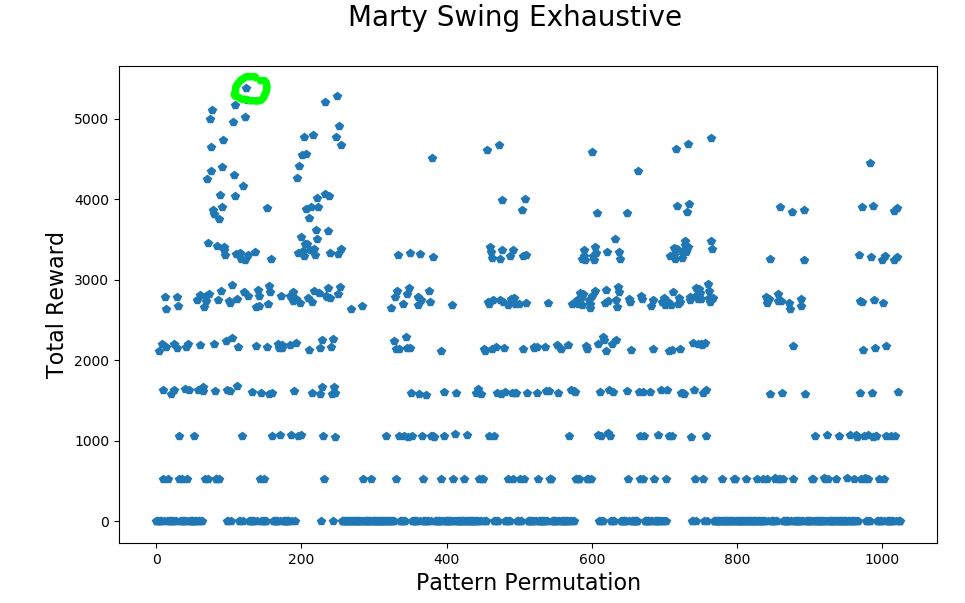 The chart above shows the result of this approach. Every one of the 1024 possible patterns was evaluated and the total reward for pattern number 124 turned out to have the highest total reward of 5380.70. Several other patterns came close too.
To see what this pattern looks like here’s the animation.

And finally, for a bit of fun, here’s what happens if we pretend that Marty could add a lot more energy in each pump. Needless to say the Swing Angle is a bit nuts as it starts adding up each rotation!

The code is on GitHub In the folder “Software/Step 6 OpenAI Machine Learning”